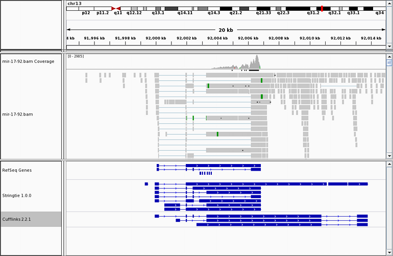
Many transcriptome assemblers have a hard time assembling transcripts
in regions where introns have been retained, even in a small percentage of transcripts. Here is an example
where RNA-seq data
from a human kidney cell line shows increased transcription activity in the region containing
the miR-17-92 cluster, one of the most potent oncogenic miRNA polycistrons. The six miRNAs
included in the miR-17-92 cluster reside inside the third intron of the MIR17HG non-coding
RNA. Read alignments across the entire span of this intron prevent other transcriptome
assemblers from assembling it correctly, but StringTie gets it right, as shown here.
The BAM alignment file (produced by TopHat2) of the RNA-seq data from this region can be downloaded
from here.
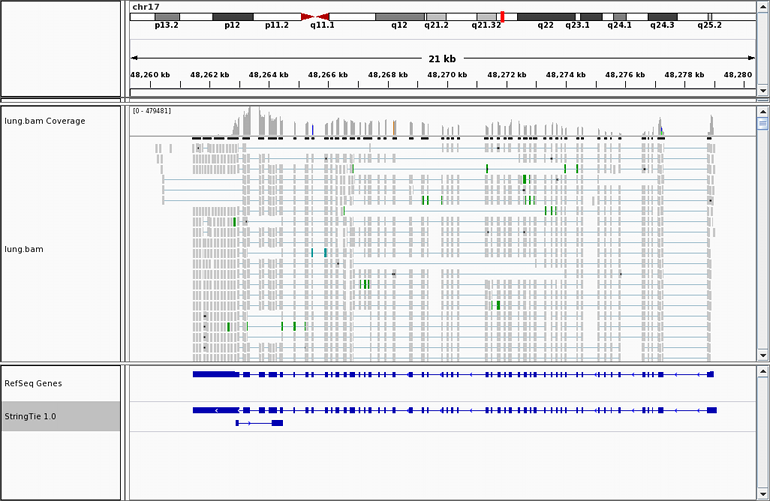
Highly covered regions pose a great challenge for transcriptome assembly and most software cannot handle them.
RNA-seq data from the cytosol of fetal lung fibroblasts (downloaded from the ENCODE data set, GEO accession GSM981244) shows a very high level of expression for the COL1A1 gene, although StringTie can still handle it. The TopHat alignment BAM file of the RNA-seq data from this region can be downloaded from here.
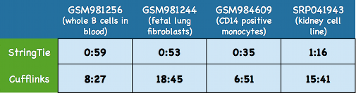
StringTie is not only accurate but also very fast compared to most other transcriptome assemblers.
Here we show some typical running times for StringTie and Cufflinks on four large real data sets including
three human RNA-seq data sets downloaded from the
ENCODE project
(GEO accessions GSM981256, GSM981244, and GSM984609) and one RNA-seq data generated from nuclear RNA
from a human kidney cell line (NCBI Study accession number
SRP041943).
Both programs were run on the same multi-core 2.1 GHz AMD Opteron servers using 8 threads.
Time is shown in as hours:minutes.
Our focus in developing StringTie was on building a system that can assemble and quantitate transcripts
regardless of whether gene annotation is available. For this task, the Cufflinks system has been the
leading method since it first appeared in 2010. In our experiments, Cufflinks consistently outperformed
all other transcriptome assemblers (except StringTie) on a variety of human RNA-seq data sets, in many
cases by a large margin. Nonetheless, StringTie consistently outperforms Cufflinks by a substantial
amount, as shown below on four real
data sets: GSM981256,
GSM981244,
GSM984609,
and SRP041943.
Note that we only show comparisons to Cufflinks because all other methods that we tested performed
considerably worse. See the forthcoming StringTie paper and its Supplement for details including comparisons to other
methods.
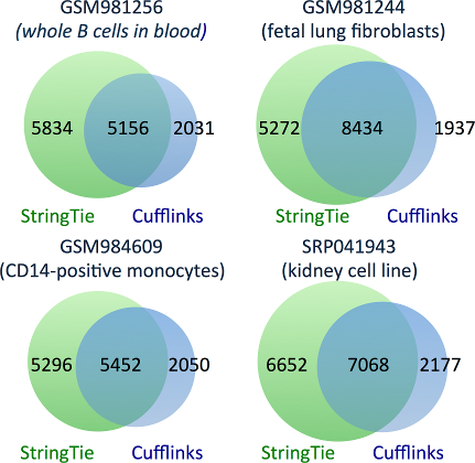
StringTie correctly assembles 32-53% more transcripts than Cufflinks.
The figure below shows Venn diagrams representing the transcripts correctly identified
by either StringTie, Cufflinks, or both. Note that this figure only counts transcripts
that precisely match known genes and are presumably correct.
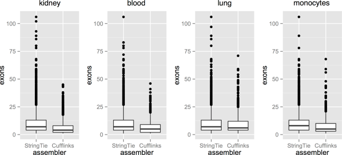
Transcripts with a larger number of exons are more likely to be assembled by StringTie rather than Cufflinks, as shown by these box and whisker diagrams that display the distribution of the number of exons in transcripts identified by StringTie and not Cufflinks, or by Cufflinks and not StringTie.
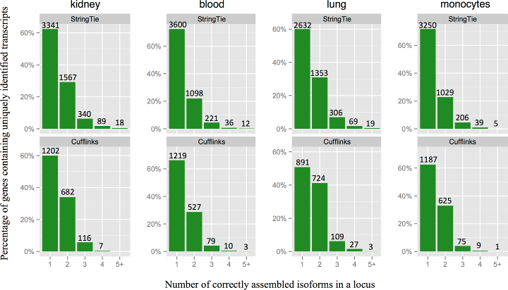
StringTie assembles a larger number of correct isoforms per gene locus.
Stringtie is an efficient tool for assembling transcriptomes and estimating expression levels. However, accuracy of the results does not depend only on the software tools, but also quality and the ammount of sequencing, which might often be expensive. It is common to be faced with a challenging tradeoff between sequencing expenses and accuracy of gene-level or transcript-level expression estimates.
We simulated RNA sequencing of human tissue transcriptomes at incremental sequencing depth. Twelve alignments (Adipose tissue, Blood vessel, Brain, Heart, Lung, Muscle, Skin, Thyroid) from the GTEx dataset were selected to maximize the number of aligned paired-end reads but also to maintain a relatively small distribution of the number of spots. Two figures below are provided as to visualize changes in expression variation, rate of false negatives and fold change associated with a lower sequencing depth.
Fig1. Plot shows an increase in variation (%TPM) associated with a lower number of reads aligned to the reference. The median (dark line), interquartile range (dark-red area) and whiskers (light-red area) are shown in the figure. High and low whiskers were computed as: and , where IQR is interquartile range, Q3 and Q1 are 3rd and 1st quartiles respectively.
Fig2. Plot shows a decrease in recall (blue) and and increase in fraction of genes with significant expression estimation change (green) associated with a lower number of aligned reads used in the assembly. Genes counted for fold change graph were selected as those having two or more fold increase or decrease in TPM from the control assembly of full set of aligned paired-end reads. Fraction of expressed genes recovered in assembly (Recall) was calculated as: .
Additional statistical evaluations (i.e. Ranking order correlations, precision and per-gene analysis) have been computed and plotted to facilitate better understanding of the dataset and changes associated with a lower sequencing depth. Information may be located in the following GitHub repository, which contains a python application developed to automate selection of alignments, assembly, statistical analysis and plotting. Readme file contains detailed instructions about the pipeline and output. All the plots generated in the experiment are also available within the figures directory on the repository.

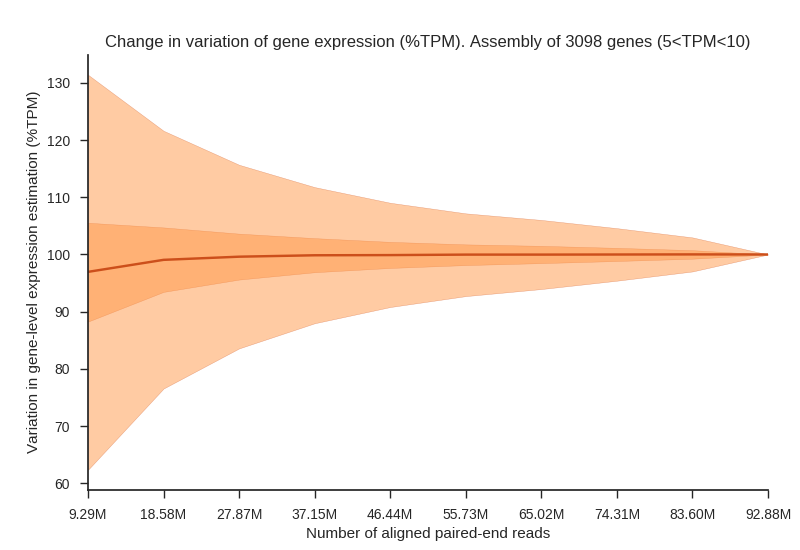
 and
and  , where IQR is interquartile range, Q3 and Q1 are 3rd and 1st quartiles respectively.
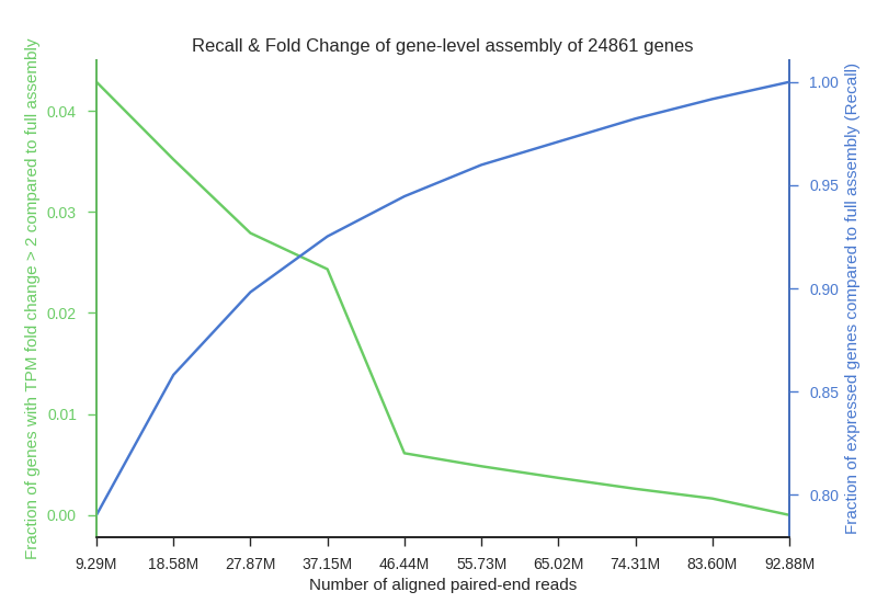
 .
.